Examples

To complement this documentation, the distribution includes a number of examples that explain how to use this software.

• two_states_dynamics.py: This example shows how the cell dynamic behaves. It compares the state probability and the transition matrix of two cells which where trained with a different set of observations. It is useful to understand the difference between a learning HMM and one with a fixed model. Also, it is a good way to analyze the impact of the eta parameter.

• three_states_dynamics.py: This example is similar to the previous one, but using a HMM with three states. Only one cell is trained and the output is one graph that shows, in the upper part, the resulting state transition matrix as a color map and in the lower part the evolution of each state probability.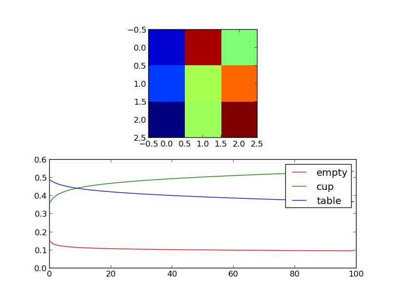

  

• mongillodeneve_test.py: This example functions as a proof that the dynamic model is correctly implemented. It reproduces a result from the paper that described the algorithm used to train the HMMs of this map. This example uses the training data in train_samples.py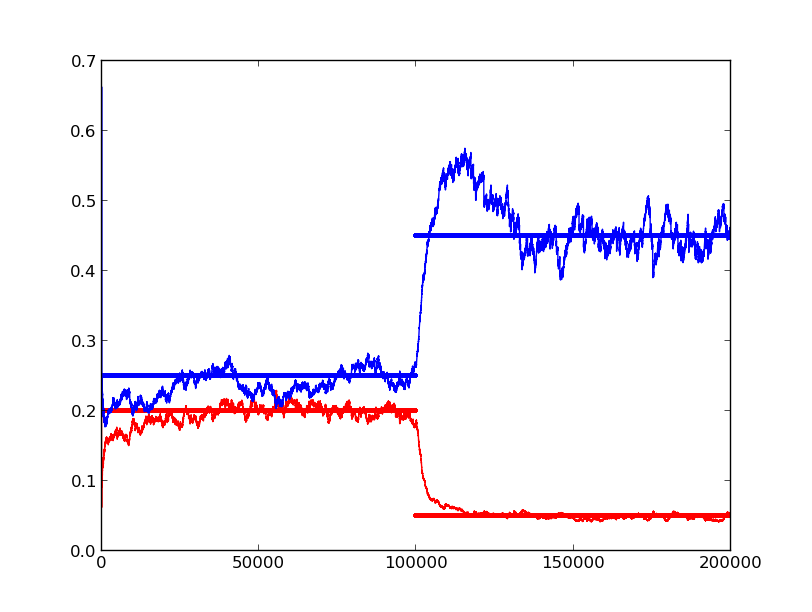

  

• two_boxes.py: This example generates a map where there are two boxes over a table. These boxes appear at different times and are removed at the same time. It shows how to use the DynamicMap API to build a map and confirms the behaviour expected after analyzing the dynamics examples. To build the map it uses generated data.

• cup_and_table.py: Similar to the previous example, but using more states than free and occ. The map is constructed with three different objects (a cup and a box over a table) and then it is queried for the most probable locations to find each element. To build the map it uses generated data. The resulting map is shown in the first image of this document.

• map_building_memory_usage.py: This example serves as a memory usage benchmark. As the space requirements can be quite big, using this example one can estimate how much memory a map will require depending on it’s size. It also serves to prove that there are no memory leaks (specially important for the C module that was written for this map).

• map_kinect_data.py: Builds a map out of 10 frames captured from a Kinect camera. The data has been pre-transformed to a list of space coordinates. It is useful as a benchmark to see how much time it is required to process and entire point cloud.

• color_boxes_from_bag.py: This is an example of a possible real world application. Kinect data is taken from a bag file provided as argument, it is then segmented according to color and the resulting point clouds are used to build a multi state map. With the generated map we can explore how the transition probabilities show the dynamics of the scene.